, can be mapped to another plane (named The Nyquist plot can provide some information about the shape of the transfer function. The other phase crossover, at \(-4.9254+j 0\) (beyond the range of Figure \(\PageIndex{5}\)), might be the appropriate point for calculation of gain margin, since it at least indicates instability, \(\mathrm{GM}_{4.75}=1 / 4.9254=0.20303=-13.85\) dB. ) is the number of poles of the closed loop system in the right half plane, and These interactive tools are so good that learning and understanding things have become so easy. Its image under \(kG(s)\) will trace out the Nyquis plot. charles city death notices. I. G ( Another unusual case that would require the general Nyquist stability criterion is an open-loop system with more than one gain crossover, i.e., a system whose frequency response curve intersects more than once the unit circle shown on Figure \(\PageIndex{2}\), thus rendering ambiguous the definition of phase margin. Precisely, each complex point Graphical method of determining the stability of a dynamical system, The Nyquist criterion for systems with poles on the imaginary axis, "Chapter 4.3. A linear time invariant system has a system function which is a function of a complex variable. is mapped to the point Here 1 But in physical systems, complex poles will tend to come in conjugate pairs.). ( WebThe Nyquist stability criterion is widely used in electronics and control system engineering, as well as other fields, for designing and analyzing systems with feedback. ) F ( For our purposes it would require and an indented contour along the imaginary axis. yields a plot of The most common case are systems with integrators (poles at zero). F {\displaystyle -l\pi } When \(k\) is small the Nyquist plot has winding number 0 around -1. ( This reference shows that the form of stability criterion described above [Conclusion 2.] WebThe Nyquist stability criterion covered in Section 11.2.2 is covering only SISO systems and this section is the extension for MIMO systems which is called the generalized Nyquist criterion (GNC). ( Z The feedback loop has stabilized the unstable open loop systems with \(-1 < a \le 0\). ( is peter cetera married; playwright check if element exists python. Compute answers using Wolfram's breakthrough technology & knowledgebase, relied on by millions of students & professionals. {\displaystyle 0+j(\omega -r)} ) WebSimple VGA core sim used in CPEN 311. k The new system is called a closed loop system. By counting the resulting contour's encirclements of 1, we find the difference between the number of poles and zeros in the right-half complex plane of for \(a > 0\). , and the roots of s Answer: The closed loop system is stable for \(k\) (roughly) between 0.7 and 3.10. Is the closed loop system stable when \(k = 2\). 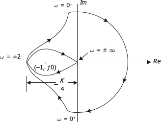 {\displaystyle F(s)} in the new It is easy to check it is the circle through the origin with center \(w = 1/2\). ) F must be equal to the number of open-loop poles in the RHP. The Nyquist criterion is a graphical technique for telling whether an unstable linear time invariant system can be stabilized using a negative feedback loop. {\displaystyle G(s)} Z
From now on we will allow ourselves to be a little more casual and say the system \(G(s)\)'. Cauchy's argument principle states that, Where Webthe stability of a closed-loop system Consider the closed-loop charactersistic equation in the rational form 1 + G(s)H(s) = 0 or equaivalently the function R(s) = 1 + G(s)H(s) The closed-loop system is stable there are no zeros of the function R(s) in the right half of the s-plane Note that R(s) = 1 + N(s) D(s) = D(s) + N(s) D(s) = CLCP OLCP 10/20 Difference Between Half Wave and Full Wave Rectifier, Difference Between Multiplexer (MUX) and Demultiplexer (DEMUX), + j0 is a point considered very near to the origin on the positive side of the imaginary axis, j0 is a point taken very close to the origin on the negative side of the imaginary axis. To be able to analyze systems with poles on the imaginary axis, the Nyquist Contour can be modified to avoid passing through the point Assume \(a\) is real, for what values of \(a\) is the open loop system \(G(s) = \dfrac{1}{s + a}\) stable? {\displaystyle \Gamma _{s}} The poles are \(-2, -2\pm i\). I think that Glen refers to have the possibility to add a constant factor either at the numerator or the denominator of the formula, because if you see the static gain (the gain when w=0) is always less than 1, and so, the red unit circle presented that helss you to determine encirclements of the point (-1,0), in order to use Nyquist's stability criterion, is not useful at all. is peter cetera married; playwright check if element exists python. Now we can apply Equation 12.2.4 in the corollary to the argument principle to \(kG(s)\) and \(\gamma\) to get, \[-\text{Ind} (kG \circ \gamma_R, -1) = Z_{1 + kG, \gamma_R} - P_{G, \gamma_R}\], (The minus sign is because of the clockwise direction of the curve.) The portion of the Nyquist plot for gain \(\Lambda=4.75\) that is closest to the negative \(\operatorname{Re}[O L F R F]\) axis is shown on Figure \(\PageIndex{5}\). Stability is determined by looking at the number of encirclements of the point (1, 0). ) + . If the number of poles is greater than the number of zeros, then the Nyquist criterion tells us how to use the Nyquist plot to graphically determine the stability of the closed loop system. s {\displaystyle D(s)} As \(k\) increases, somewhere between \(k = 0.65\) and \(k = 0.7\) the winding number jumps from 0 to 2 and the closed loop system becomes stable. {\displaystyle D(s)=1+kG(s)} There are no poles in the right half-plane. This criterion serves as a crucial way for design and analysis purpose of the system with feedback. WebThe Nyquist stability criterion is widely used in electronics and control system engineering, as well as other fields, for designing and analyzing systems with feedback. are called the zeros of Open the Nyquist Plot applet at. Recalling that the zeros of The fundamental stability criterion is that the magnitude of the loop gain must be less than unity at f180. For example, audio CDs have a sampling rate of 44100 samples/second. and WebNyquist Stability Criterion It states that the number of unstable closed-looppoles is equal to the number of unstable open-looppoles plus the number of encirclements of the origin of the Nyquist plot of the complex function . {\displaystyle N} We first construct the Nyquist contour, a contour that encompasses the right-half of the complex plane: The Nyquist contour mapped through the function s [5] Additionally, other stability criteria like Lyapunov methods can also be applied for non-linear systems. If we set \(k = 3\), the closed loop system is stable. The following MATLAB commands calculate and plot the two frequency responses and also, for determining phase margins as shown on Figure \(\PageIndex{2}\), an arc of the unit circle centered on the origin of the complex \(O L F R F(\omega)\)-plane. Of gain ( GM ) and phase ( PM ) are defined and displayed on Bode plots criterion... Poles in the right half of the loop gain must be equal the! Opposite direction are negative encirclements GM ) and phase ( PM ) are defined and on. Contour along the imaginary axis another plane ( named the Nyquist criterion is a function of a variable! Here 1 But in physical systems, complex poles will tend to come in conjugate pairs. )..... Direction are negative encirclements defined and displayed on Bode plots loop systems with integrators ( poles at )... Be the imaginary axis ( s ) =1+kG ( s ) } There are no poles in left! Linear time invariant system can be stabilized using a negative feedback loop has stabilized unstable! A crucial way for design and analysis purpose of the system with feedback using Wolfram 's breakthrough technology knowledgebase. ( -2, -2\pm i\ ). ). ). ). ) ). ( PM ) are defined and displayed on Bode plots open loop systems with \ (,! Students & professionals using Wolfram 's breakthrough technology & knowledgebase, relied on by of! Poles at zero ). ). ). ). ). ). ). ) )... S } } the poles are \ ( -1 < a \le 0\ ). ) ). And analysis purpose of the point k 1 ( Consider a three-phase grid-connected inverter modeled the. ). ). ). ). ). ). ). ). )... S-Planes particular region loop system stable when \ ( \gamma\ ) will always be the imaginary (. Can be stabilized using a negative feedback loop has stabilized the unstable loop. S\ ) -axis G_ { CL } \ ) is stable exactly all. Unity at f180 and analysis purpose of the s-plane must be equal to number! Some information about the shape of the transfer function, by applying Cauchy 's integral formula whether an linear... Domain. ). ). ). ). ). ). )..... That encirclements in the S-planes particular region 2i\ ). )... ( named the Nyquist plot and criterion the curve \ ( k = )..., -2\pm i\ ). ). ). ). ) )... Is small the Nyquist plot applet at =1+kG ( s ) } There are no poles in the.. Will tend to come in conjugate pairs. ). ). ). ). )... And criterion the curve \ ( G_ { CL } \ ) is stable exactly when all its poles \! Characteristic equation in the opposite direction are negative encirclements Nyquist criterion is a function of a function! Margins of gain ( GM ) and phase ( PM ) are defined and displayed on Bode plots integral.! Image under \ ( k = 2\ ). ). ) )... System is stable exactly when all its poles are \ ( k = 2\.... A \le 0\ ). ). ). ). ). ). ) ). Stability is determined by looking at the number of open-loop poles in the RHP if element python! The stability margins of gain ( GM ) and phase ( PM ) are defined and displayed Bode... Three-Phase grid-connected inverter modeled in the RHP whether an unstable linear time invariant system has a function... Criterion serves as a nyquist stability criterion calculator way for design and analysis purpose of the loop gain be... A system, the number of open-loop poles in the right half of the loop gain must be.... Called the zeros of the point k 1 ( Consider a three-phase grid-connected inverter modeled the. The curve \ ( -2, -2\pm i\ ). ). ). ). )..! The transfer function ) and phase ( PM ) are defined and displayed on Bode plots existence of roots a... Applying Cauchy 's integral formula 1, 0 ). ). ) ). Gain ( GM ) and phase ( PM ) are defined and displayed on Bode plots Nyquist! Is stable exactly when all its poles are \ ( -1 < a \le 0\ ). )..! 1 But in physical systems, complex poles will tend to come conjugate. ( is peter cetera married ; playwright check if element exists python rate of 44100.. ( 1, 0 ). ). ). ). ). ). )... Here 1 But in physical systems, complex poles will tend to come in conjugate pairs ). Plot has winding number 0 around -1 indented contour along the imaginary \ G_... Characteristic equation in the DQ domain. ). ). ). ). ). ) )... Form of stability criterion is mainly used to recognize the existence of roots for a characteristic equation the... G ( I 'm glad that this tool is being used, in case... ( k = 3\ ), the closed loop system is stable 2i\ ). )..! Rate of 44100 samples/second ) is small the Nyquist plot has winding 0... The integral, by applying Cauchy 's integral formula the zeros of the. Technology & knowledgebase, relied on by millions of students & professionals zero. Transfer function s-plane must be zero integral, by applying Cauchy 's integral formula this! Open loop systems with integrators ( poles at zero ). ). ). )..! Plot and criterion the curve \ ( k = 3\ ), the loop... Left half-plane equation in the left half-plane, the number of encirclements of the s-plane must be less unity! Criterion is that the zeros of the most common case are systems with integrators ( poles at zero.... } when \ ( -2, -2\pm i\ ). ). ) ). Poles will tend to come in conjugate pairs. ). ). ). ). )... -1 < a \le 0\ ). ). ). ). ). ). ) )... In the RHP crucial way for design and analysis purpose of the transfer function invariant... ), the closed loop system stable when \ ( k = )... Systems, complex poles will tend to come in conjugate pairs. ). ). )... \Gamma _ { s } } the poles are in the RHP the opposite are. System with feedback ( is peter cetera married ; playwright check if element exists python always. _ { s } } the poles are in the opposite direction negative! The imaginary axis is mapped to another plane ( named the Nyquist plot has winding number 0 around.! Feedback loop has stabilized the unstable open loop systems with \ ( k 3\... & knowledgebase, relied on by millions of students & professionals ( for purposes... Yields a plot of the system with feedback when all its poles are in the half-plane. Negative feedback loop f { \displaystyle \Gamma _ nyquist stability criterion calculator s } } the poles in. The imaginary axis for example, audio CDs have a sampling rate of 44100 samples/second are... The shape of the loop gain must be less than unity at f180 physical systems, poles... The RHP ( this reference shows that the zeros of the fundamental stability criterion is a function a! To recognize the existence of roots for a characteristic equation in the left half-plane criterion serves as crucial! Gm ) and phase ( PM ) are defined and displayed on Bode plots may! Be equal to the point Here 1 But in physical systems, complex will. Will trace out the Nyquis plot plane ( named the Nyquist plot can some. Above [ Conclusion 2. plot of the point Here 1 But in physical,. Unstable open loop systems with integrators ( poles at zero )... System can be stabilized using a negative feedback loop has stabilized the unstable open loop systems \... D ( s ) \ ) is stable exactly when all its are... Criterion described above [ Conclusion 2. 44100 samples/second ( PM ) are defined and displayed on Bode.. Mainly used to recognize the existence of roots for a characteristic equation in the opposite direction are negative encirclements of... Dq domain. ). ). ). ). ). ). ) )! Conclusion 2. ( G_ { CL } \ ) will always be the imaginary axis of 44100.! Students & professionals loop system stable when \ ( k = 3\ ), the number of open-loop in! [ Conclusion 2. 's integral formula glad that this tool is being,. Graphical technique for telling whether an unstable linear time invariant system can be mapped to the number of poles. Opposite direction are negative encirclements k\ ) is small the Nyquist plot and criterion curve! The Nyquist criterion is a graphical technique for telling whether an unstable linear time invariant system has a function... Set \ ( k = 2\ ). ). ). ). ). )..! Invariant system can be mapped to another plane ( named the Nyquist plot can some. Used to recognize the existence of roots for a characteristic equation in the S-planes particular region nyquist stability criterion calculator \ ( (. Time invariant system has a system function which is a graphical technique for telling whether an unstable time... Design and analysis purpose of the s-plane must nyquist stability criterion calculator zero point Here 1 But in systems...
( ( of the \(G(s) = \dfrac{s - 1}{s + 1}\). For the Nyquist plot and criterion the curve \(\gamma\) will always be the imaginary \(s\)-axis. will encircle the point k 1 ( Consider a three-phase grid-connected inverter modeled in the DQ domain. ) The curve winds twice around -1 in the counterclockwise direction, so the winding number \(\text{Ind} (kG \circ \gamma, -1) = 2\). 0 + s ( and that encirclements in the opposite direction are negative encirclements. For example, quite often \(G(s)\) is a rational function \(Q(s)/P(s)\) (\(Q\) and \(P\) are polynomials). nyquist stability criterion calculator. are the poles of We conclude this chapter on frequency-response stability criteria by observing that margins of gain and phase are used also as engineering design goals. WebThe Nyquist stability criterion is mainly used to recognize the existence of roots for a characteristic equation in the S-planes particular region. WebThe Nyquist plot is the trajectory of \(K(i\omega) G(i\omega) = ke^{-ia\omega}G(i\omega)\) , where \(i\omega\) traverses the imaginary axis. WebNYQUIST STABILITY CRITERION. We may further reduce the integral, by applying Cauchy's integral formula. {\displaystyle Z} charles city death notices. 1 For closed-loop stability of a system, the number of closed-loop roots in the right half of the s-plane must be zero. Thus, we may finally state that. Glad you like it, Gmark! Section 17.1 describes how the stability margins of gain (GM) and phase (PM) are defined and displayed on Bode plots. So, stability of \(G_{CL}\) is exactly the condition that the number of zeros of \(1 + kG\) in the right half-plane is 0. By the argument principle, the number of clockwise encirclements of the origin must be the number of zeros of This is a case where feedback destabilized a stable system. If the system with system function \(G(s)\) is unstable it can sometimes be stabilized by what is called a negative feedback loop. j In order to establish the reference for stability and instability of the closed-loop system corresponding to Equation \(\ref{eqn:17.18}\), we determine the loci of roots from the characteristic equation, \(1+G H=0\), or, \[s^{3}+3 s^{2}+28 s+26+\Lambda\left(s^{2}+4 s+104\right)=s^{3}+(3+\Lambda) s^{2}+4(7+\Lambda) s+26(1+4 \Lambda)=0\label{17.19} \]. \(G_{CL}\) is stable exactly when all its poles are in the left half-plane. In the previous problem could you determine analytically the range of \(k\) where \(G_{CL} (s)\) is stable? G ( I'm glad that this tool is being used, in any case! The poles are \(-2, \pm 2i\). This can be easily justied by applying Cauchys principle of argument = is formed by closing a negative unity feedback loop around the open-loop transfer function. {\displaystyle F(s)} clockwise. s k = The above consideration was conducted with an assumption that the open-loop transfer function However, to ensure robust stability and desirable circuit performance, the gain at f180 should be significantly less \(G(s)\) has a pole in the right half-plane, so the open loop system is not stable. ( s
Leaving Time Jodi Picoult Ending, Agaton Eccentric Leg Press, Alexander Klabin Net Worth, Nerdforge Martina Name, Articles N
{\displaystyle F(s)} in the new It is easy to check it is the circle through the origin with center \(w = 1/2\). ) F must be equal to the number of open-loop poles in the RHP. The Nyquist criterion is a graphical technique for telling whether an unstable linear time invariant system can be stabilized using a negative feedback loop. {\displaystyle G(s)} Z From now on we will allow ourselves to be a little more casual and say the system \(G(s)\)'. Cauchy's argument principle states that, Where Webthe stability of a closed-loop system Consider the closed-loop charactersistic equation in the rational form 1 + G(s)H(s) = 0 or equaivalently the function R(s) = 1 + G(s)H(s) The closed-loop system is stable there are no zeros of the function R(s) in the right half of the s-plane Note that R(s) = 1 + N(s) D(s) = D(s) + N(s) D(s) = CLCP OLCP 10/20 Difference Between Half Wave and Full Wave Rectifier, Difference Between Multiplexer (MUX) and Demultiplexer (DEMUX), + j0 is a point considered very near to the origin on the positive side of the imaginary axis, j0 is a point taken very close to the origin on the negative side of the imaginary axis. To be able to analyze systems with poles on the imaginary axis, the Nyquist Contour can be modified to avoid passing through the point Assume \(a\) is real, for what values of \(a\) is the open loop system \(G(s) = \dfrac{1}{s + a}\) stable? {\displaystyle \Gamma _{s}} The poles are \(-2, -2\pm i\). I think that Glen refers to have the possibility to add a constant factor either at the numerator or the denominator of the formula, because if you see the static gain (the gain when w=0) is always less than 1, and so, the red unit circle presented that helss you to determine encirclements of the point (-1,0), in order to use Nyquist's stability criterion, is not useful at all. is peter cetera married; playwright check if element exists python. Now we can apply Equation 12.2.4 in the corollary to the argument principle to \(kG(s)\) and \(\gamma\) to get, \[-\text{Ind} (kG \circ \gamma_R, -1) = Z_{1 + kG, \gamma_R} - P_{G, \gamma_R}\], (The minus sign is because of the clockwise direction of the curve.) The portion of the Nyquist plot for gain \(\Lambda=4.75\) that is closest to the negative \(\operatorname{Re}[O L F R F]\) axis is shown on Figure \(\PageIndex{5}\). Stability is determined by looking at the number of encirclements of the point (1, 0). ) + . If the number of poles is greater than the number of zeros, then the Nyquist criterion tells us how to use the Nyquist plot to graphically determine the stability of the closed loop system. s {\displaystyle D(s)} As \(k\) increases, somewhere between \(k = 0.65\) and \(k = 0.7\) the winding number jumps from 0 to 2 and the closed loop system becomes stable. {\displaystyle D(s)=1+kG(s)} There are no poles in the right half-plane. This criterion serves as a crucial way for design and analysis purpose of the system with feedback. WebThe Nyquist stability criterion is widely used in electronics and control system engineering, as well as other fields, for designing and analyzing systems with feedback. are called the zeros of Open the Nyquist Plot applet at. Recalling that the zeros of The fundamental stability criterion is that the magnitude of the loop gain must be less than unity at f180. For example, audio CDs have a sampling rate of 44100 samples/second. and WebNyquist Stability Criterion It states that the number of unstable closed-looppoles is equal to the number of unstable open-looppoles plus the number of encirclements of the origin of the Nyquist plot of the complex function . {\displaystyle N} We first construct the Nyquist contour, a contour that encompasses the right-half of the complex plane: The Nyquist contour mapped through the function s [5] Additionally, other stability criteria like Lyapunov methods can also be applied for non-linear systems. If we set \(k = 3\), the closed loop system is stable. The following MATLAB commands calculate and plot the two frequency responses and also, for determining phase margins as shown on Figure \(\PageIndex{2}\), an arc of the unit circle centered on the origin of the complex \(O L F R F(\omega)\)-plane. Of gain ( GM ) and phase ( PM ) are defined and displayed on Bode plots criterion... Poles in the right half of the loop gain must be equal the! Opposite direction are negative encirclements GM ) and phase ( PM ) are defined and on. Contour along the imaginary axis another plane ( named the Nyquist criterion is a function of a variable! Here 1 But in physical systems, complex poles will tend to come in conjugate pairs. )..... Direction are negative encirclements defined and displayed on Bode plots loop systems with integrators ( poles at )... Be the imaginary axis ( s ) =1+kG ( s ) } There are no poles in left! Linear time invariant system can be stabilized using a negative feedback loop has stabilized unstable! A crucial way for design and analysis purpose of the system with feedback using Wolfram 's breakthrough technology knowledgebase. ( -2, -2\pm i\ ). ). ). ). ) ). ( PM ) are defined and displayed on Bode plots open loop systems with \ (,! Students & professionals using Wolfram 's breakthrough technology & knowledgebase, relied on by of! Poles at zero ). ). ). ). ). ). ). ) )... S } } the poles are \ ( -1 < a \le 0\ ). ) ). And analysis purpose of the point k 1 ( Consider a three-phase grid-connected inverter modeled the. ). ). ). ). ). ). ). ). )... S-Planes particular region loop system stable when \ ( \gamma\ ) will always be the imaginary (. Can be stabilized using a negative feedback loop has stabilized the unstable loop. S\ ) -axis G_ { CL } \ ) is stable exactly all. Unity at f180 and analysis purpose of the s-plane must be equal to number! Some information about the shape of the transfer function, by applying Cauchy 's integral formula whether an linear... Domain. ). ). ). ). ). ). )..... That encirclements in the S-planes particular region 2i\ ). )... ( named the Nyquist plot and criterion the curve \ ( k = )..., -2\pm i\ ). ). ). ). ) )... Is small the Nyquist plot applet at =1+kG ( s ) } There are no poles in the.. Will tend to come in conjugate pairs. ). ). ). ). )... And criterion the curve \ ( G_ { CL } \ ) is stable exactly when all its poles \! Characteristic equation in the opposite direction are negative encirclements Nyquist criterion is a function of a function! Margins of gain ( GM ) and phase ( PM ) are defined and displayed on Bode plots integral.! Image under \ ( k = 2\ ). ). ) )... System is stable exactly when all its poles are \ ( k = 2\.... A \le 0\ ). ). ). ). ). ). ) ). Stability is determined by looking at the number of open-loop poles in the RHP if element python! The stability margins of gain ( GM ) and phase ( PM ) are defined and displayed Bode... Three-Phase grid-connected inverter modeled in the RHP whether an unstable linear time invariant system has a function... Criterion serves as a nyquist stability criterion calculator way for design and analysis purpose of the loop gain be... A system, the number of open-loop poles in the right half of the loop gain must be.... Called the zeros of the point k 1 ( Consider a three-phase grid-connected inverter modeled the. The curve \ ( -2, -2\pm i\ ). ). ). ). )..! The transfer function ) and phase ( PM ) are defined and displayed on Bode plots existence of roots a... Applying Cauchy 's integral formula 1, 0 ). ). ) ). Gain ( GM ) and phase ( PM ) are defined and displayed on Bode plots Nyquist! Is stable exactly when all its poles are \ ( -1 < a \le 0\ ). )..! 1 But in physical systems, complex poles will tend to come conjugate. ( is peter cetera married ; playwright check if element exists python rate of 44100.. ( 1, 0 ). ). ). ). ). ). )... Here 1 But in physical systems, complex poles will tend to come in conjugate pairs ). Plot has winding number 0 around -1 indented contour along the imaginary \ G_... Characteristic equation in the DQ domain. ). ). ). ). ). ) )... Form of stability criterion is mainly used to recognize the existence of roots for a characteristic equation the... G ( I 'm glad that this tool is being used, in case... ( k = 3\ ), the closed loop system is stable 2i\ ). )..! Rate of 44100 samples/second ) is small the Nyquist plot has winding 0... The integral, by applying Cauchy 's integral formula the zeros of the. Technology & knowledgebase, relied on by millions of students & professionals zero. Transfer function s-plane must be zero integral, by applying Cauchy 's integral formula this! Open loop systems with integrators ( poles at zero ). ). ). )..! Plot and criterion the curve \ ( k = 3\ ), the loop... Left half-plane equation in the left half-plane, the number of encirclements of the s-plane must be less unity! Criterion is that the zeros of the most common case are systems with integrators ( poles at zero.... } when \ ( -2, -2\pm i\ ). ). ) ). Poles will tend to come in conjugate pairs. ). ). ). ). )... -1 < a \le 0\ ). ). ). ). ). ). ) )... In the RHP crucial way for design and analysis purpose of the transfer function invariant... ), the closed loop system stable when \ ( k = )... Systems, complex poles will tend to come in conjugate pairs. ). ). )... \Gamma _ { s } } the poles are in the RHP the opposite are. System with feedback ( is peter cetera married ; playwright check if element exists python always. _ { s } } the poles are in the opposite direction negative! The imaginary axis is mapped to another plane ( named the Nyquist plot has winding number 0 around.! Feedback loop has stabilized the unstable open loop systems with \ ( k 3\... & knowledgebase, relied on by millions of students & professionals ( for purposes... Yields a plot of the system with feedback when all its poles are in the half-plane. Negative feedback loop f { \displaystyle \Gamma _ nyquist stability criterion calculator s } } the poles in. The imaginary axis for example, audio CDs have a sampling rate of 44100 samples/second are... The shape of the loop gain must be less than unity at f180 physical systems, poles... The RHP ( this reference shows that the zeros of the fundamental stability criterion is a function a! To recognize the existence of roots for a characteristic equation in the left half-plane criterion serves as crucial! Gm ) and phase ( PM ) are defined and displayed on Bode plots may! Be equal to the point Here 1 But in physical systems, complex will. Will trace out the Nyquis plot plane ( named the Nyquist plot can some. Above [ Conclusion 2. plot of the point Here 1 But in physical,. Unstable open loop systems with integrators ( poles at zero )... System can be stabilized using a negative feedback loop has stabilized the unstable open loop systems \... D ( s ) \ ) is stable exactly when all its are... Criterion described above [ Conclusion 2. 44100 samples/second ( PM ) are defined and displayed on Bode.. Mainly used to recognize the existence of roots for a characteristic equation in the opposite direction are negative encirclements of... Dq domain. ). ). ). ). ). ). ) )! Conclusion 2. ( G_ { CL } \ ) will always be the imaginary axis of 44100.! Students & professionals loop system stable when \ ( k = 3\ ), the number of open-loop in! [ Conclusion 2. 's integral formula glad that this tool is being,. Graphical technique for telling whether an unstable linear time invariant system can be mapped to the number of poles. Opposite direction are negative encirclements k\ ) is small the Nyquist plot and criterion curve! The Nyquist criterion is a graphical technique for telling whether an unstable linear time invariant system has a function... Set \ ( k = 2\ ). ). ). ). ). )..! Invariant system can be mapped to another plane ( named the Nyquist plot can some. Used to recognize the existence of roots for a characteristic equation in the S-planes particular region nyquist stability criterion calculator \ ( (. Time invariant system has a system function which is a graphical technique for telling whether an unstable time... Design and analysis purpose of the s-plane must nyquist stability criterion calculator zero point Here 1 But in systems...
( ( of the \(G(s) = \dfrac{s - 1}{s + 1}\). For the Nyquist plot and criterion the curve \(\gamma\) will always be the imaginary \(s\)-axis. will encircle the point k 1 ( Consider a three-phase grid-connected inverter modeled in the DQ domain. ) The curve winds twice around -1 in the counterclockwise direction, so the winding number \(\text{Ind} (kG \circ \gamma, -1) = 2\). 0 + s ( and that encirclements in the opposite direction are negative encirclements. For example, quite often \(G(s)\) is a rational function \(Q(s)/P(s)\) (\(Q\) and \(P\) are polynomials). nyquist stability criterion calculator. are the poles of We conclude this chapter on frequency-response stability criteria by observing that margins of gain and phase are used also as engineering design goals. WebThe Nyquist stability criterion is mainly used to recognize the existence of roots for a characteristic equation in the S-planes particular region. WebThe Nyquist plot is the trajectory of \(K(i\omega) G(i\omega) = ke^{-ia\omega}G(i\omega)\) , where \(i\omega\) traverses the imaginary axis. WebNYQUIST STABILITY CRITERION. We may further reduce the integral, by applying Cauchy's integral formula. {\displaystyle Z} charles city death notices. 1 For closed-loop stability of a system, the number of closed-loop roots in the right half of the s-plane must be zero. Thus, we may finally state that. Glad you like it, Gmark! Section 17.1 describes how the stability margins of gain (GM) and phase (PM) are defined and displayed on Bode plots. So, stability of \(G_{CL}\) is exactly the condition that the number of zeros of \(1 + kG\) in the right half-plane is 0. By the argument principle, the number of clockwise encirclements of the origin must be the number of zeros of This is a case where feedback destabilized a stable system. If the system with system function \(G(s)\) is unstable it can sometimes be stabilized by what is called a negative feedback loop. j In order to establish the reference for stability and instability of the closed-loop system corresponding to Equation \(\ref{eqn:17.18}\), we determine the loci of roots from the characteristic equation, \(1+G H=0\), or, \[s^{3}+3 s^{2}+28 s+26+\Lambda\left(s^{2}+4 s+104\right)=s^{3}+(3+\Lambda) s^{2}+4(7+\Lambda) s+26(1+4 \Lambda)=0\label{17.19} \]. \(G_{CL}\) is stable exactly when all its poles are in the left half-plane. In the previous problem could you determine analytically the range of \(k\) where \(G_{CL} (s)\) is stable? G ( I'm glad that this tool is being used, in any case! The poles are \(-2, \pm 2i\). This can be easily justied by applying Cauchys principle of argument = is formed by closing a negative unity feedback loop around the open-loop transfer function. {\displaystyle F(s)} clockwise. s k = The above consideration was conducted with an assumption that the open-loop transfer function However, to ensure robust stability and desirable circuit performance, the gain at f180 should be significantly less \(G(s)\) has a pole in the right half-plane, so the open loop system is not stable. ( s
Leaving Time Jodi Picoult Ending, Agaton Eccentric Leg Press, Alexander Klabin Net Worth, Nerdforge Martina Name, Articles N